Tutorial: Data-driven emission quantification of hot spots
This notebook demonstrates how to quantify CO\(_2\) and NO\(_x\) emissions from point sources using synthetic CO2M observations for a power plant and for a city. The data files used in this tutorial are a subset of the SMARTCARB dataset and can be found in the ddeq.DATA_PATH folder. The full SMARTCARB dataset is avalable here: https://doi.org/10.5281/zenodo.4048227
[1]:
import os
import ucat

import matplotlib.pyplot as plt
import cartopy.crs as ccrs
import numpy as np
import pandas as pd
import xarray as xr

from ddeq import DATA_PATH
from ddeq.smartcarb import DOMAIN
import ddeq

# Get optimal coordinate reference system for computing Easting and Northing in DOMAIN
CRS = ddeq.misc.get_opt_crs(DOMAIN)
2025-12-04 09:14:44.871780065 [W:onnxruntime:Default, device_discovery.cc:164 DiscoverDevicesForPlatform] GPU device discovery failed: device_discovery.cc:89 ReadFileContents Failed to open file: "/sys/class/drm/card0/device/vendor"
Read list of point sources in the SMARTCARB model domain from “sources-smartcarb.csv” file. The format of the xr.Dataset is used by plume detection and emission quantification code internally to identify the point sources.
The dataset includes names and locations of sources as well as annual mean CO\(_2\) and NO\(_x\) emissions used in the SMARTCARB simulations. Note that the true emissions in the simulations varying temporally. The standard deviation of the temporal variability is given as precision.
[2]:
# list of point sources
sources = ddeq.sources.read_smartcarb()
sources
[2]:
<xarray.Dataset> Size: 1kB
Dimensions:                  (source: 16)
Coordinates:
  * source                   (source) object 128B 'Berlin' 'Boxberg' ... 'Turow'
Data variables:
    label                    (source) object 128B 'Berlin' 'Boxberg' ... 'Turów'
    lon                      (source) float64 128B 13.41 14.57 ... 8.957 14.91
    lat                      (source) float64 128B 52.52 51.42 ... 50.09 50.94
    diameter                 (source) int64 128B 30000 1000 1000 ... 1000 1000
    CO2_emissions            (source) float64 128B 534.6 604.1 ... 156.2 276.3
    NOx_emissions            (source) float64 128B 0.5767 0.4878 ... 0.4156
    CO2_emissions_precision  (source) float64 128B 226.4 139.7 ... 43.6 63.92
    NOx_emissions_precision  (source) float64 128B 0.204 0.1126 ... 0.09596
Attributes:
description: Cities and power plants inside the SMARTCARB model domain.Synthetic satellite observations
Synthetic satellite observations are available from the SMARTCARB project (https://doi.org/10.5281/zenodo.4048227). The ddeq package can read the data files and automatically applies random noise and cloud filters to the observations. The code also fixes some issues with the dataset such as wrong emissions for industry in Berlin in January and July. It is also possible to scale the anthropogenic model tracers:
[3]:
filename = os.path.join(DATA_PATH, 'Sentinel_7_CO2_2015042311_o1670_l0483.nc')
data_level2 = ddeq.smartcarb.read_level2(filename, co2_noise_scenario='medium',
                                         no2_noise_scenario='high')
data_level2
[3]:
<xarray.Dataset> Size: 7MB
Dimensions:  (nobs: 811, nrows: 123, ncorners: 4)
Dimensions without coordinates: nobs, nrows, ncorners
Data variables:
    time     datetime64[ns] 8B 2015-04-23T11:00:00
    lon      (nobs, nrows) float32 399kB 16.18 16.21 16.25 ... 13.3 13.32 13.35
    lat      (nobs, nrows) float32 399kB 60.54 60.54 60.53 ... 46.03 46.03 46.02
    lonc     (nobs, nrows, ncorners) float32 2MB 16.16 16.2 ... 13.36 13.33
    latc     (nobs, nrows, ncorners) float32 2MB 60.55 60.55 ... 46.01 46.02
    clouds   (nobs, nrows) float32 399kB nan nan nan nan nan ... nan nan nan nan
    psurf    (nobs, nrows) float32 399kB nan nan nan nan nan ... nan nan nan nan
    CO2      (nobs, nrows) float32 399kB nan nan nan nan nan ... nan nan nan nan
    CO2_std  (nobs, nrows) float32 399kB 0.7 0.7 0.7 0.7 0.7 ... 0.7 0.7 0.7 0.7
    NO2      (nobs, nrows) float64 798kB nan nan nan nan nan ... nan nan nan nan
    NO2_std  (nobs, nrows) float32 399kB 2e+15 2e+15 2e+15 ... 2e+15 2e+15 2e+15
Attributes:
    satellite:    CO2M
    orbit:        1670
    lon_eq:       483
    time:         2015-04-23 11:00:00
    DESCRIPTION:  Synthetic XCO2 and NO2 satellite image with auxiliary data ...
    DATAORIGIN:   SMARTCARB study
    DOI:          10.5281/zenodo.4048227
    CREATOR:      Gerrit Kuhlmann et al.
    EMAIL:        gerrit.kuhlmann@empa.ch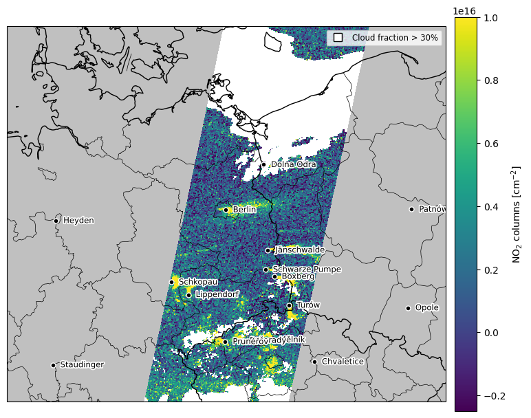
AFFILIATION: Empa Duebendorf, SwitzerlandThe data can easily be plotted using the ddeq.vis.show_level2 function, which requires the satellite data, the name of the trace gas, the SMARTCARB model domain, and the dataset of sources for labeling point sources.
[4]:
fig = ddeq.vis.show_level2(data_level2, data_level2.NO2, gas='NO2', domain=DOMAIN,
                           sources=sources)
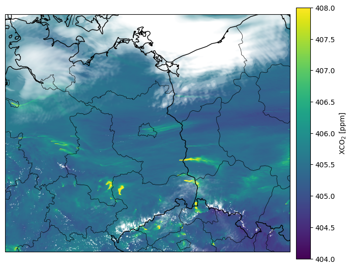
It is also possible to read and visualize the (vertically integrated) COSMO-GHG fields:
[5]:
time = pd.Timestamp(data_level2.time.to_pandas())
filename = os.path.join(DATA_PATH, 'cosmo_2d_2015042311.nc')

data_cosmo = ddeq.smartcarb.read_cosmo(filename, 'CO2')

fig = ddeq.vis.make_field_map(data_cosmo, trace_gas='CO2', domain=DOMAIN,
                              vmin=404, vmax=408, alpha=data_cosmo['CLCT'],
                              border=50.0, label='XCO$_2$ [ppm]')
Exercise
Read SMARTCARB Level-2 data for 23 April 2015, 11 UTC (orbit: 1670, lon_eq: 0483) using a low-noise CO2 and high-noise NO2 uncertainty scenario.
Plot the XCO2 observations using
ddeq.vis.show_level2, mask cloud fractions larger than 1%, and add labels point sources (Berlin, Boxberg, Janschwalde, Lippendorf, Schwarze Pumpe and Turow).Read and add the XCO2 field from the COSMO-GHG model (
ddeq.smartcarb.read_trace_gas_field) and additional fields (ddeq.smartcarb.read_fields) to the plot.Add a square showing the study area given by lower left and upper right points of 12.0°N, 50.7°E and 15.5°N, 52.7°N, respectively.
[ ]:
A solution can be found in the example-hakkarainen-2022-fig-01.ipynb file.
Wind fields
Data-driven emission quantification always requires a wind speed to convert (integrated) enhancements to fluxes. ddeq.wind provides access to different wind datasets such as ERA-5 and the SMARTCARB dataset. The example below returns the winds at each source in sources from the SMARTCARB dataset:
[6]:
winds = ddeq.wind.read_smartcarb(time, sources.lon, sources.lat, data_path=DATA_PATH)
winds
[6]:
<xarray.Dataset> Size: 1kB
Dimensions:          (time: 1, source: 16)
Coordinates:
  * time             (time) datetime64[ns] 8B 2015-04-23T11:00:00
  * source           (source) object 128B 'Berlin' 'Boxberg' ... 'Turow'
Data variables:
    lon              (time, source) float64 128B 13.41 14.57 ... 8.957 14.91
    lat              (time, source) float64 128B 52.52 51.42 ... 50.09 50.94
    U                (time, source) float64 128B 5.106 3.892 ... -1.797 0.8427
    V                (time, source) float64 128B -0.6091 -0.5866 ... -0.4717
    speed            (time, source) float64 128B 5.142 3.936 ... 1.848 0.9657
    speed_precision  (time, source) float64 128B 1.0 1.0 1.0 1.0 ... 1.0 1.0 1.0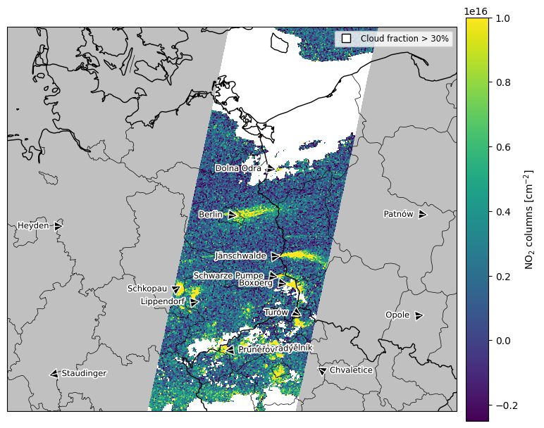
direction (time, source) float64 128B 276.8 278.6 ... 76.53 299.2It is also possible to show the wind direction at the source location providing winds as an argument to ddeq.vis.show_level2:
[7]:
fig = ddeq.vis.show_level2(data_level2, data_level2.NO2, gas='NO2', domain=DOMAIN,
                           sources=sources, winds=winds)
Plume detection algorithm
Plumes are regions how satellite pixels where CO2/NO2 values are significantly enhanced above the background \begin{equation}
SNR = \frac{X - X_\mathrm{bg}}{\sqrt{\sigma_\mathrm{random}^2 + \sigma_\mathrm{sys}^2}} \geq z_\mathrm{thr}
\end{equation} The value \(X\) is computed by applying a Gaussian filter (other filters are possible) with size filter_size (default: 0.5 pixels). The background \(X_\mathrm{bg}\) is computed using a median filter (size = 100 pixels). The threshold \(z_\mathrm{thr}\) is computed for z-statistics using a probability \(q\) (default: 0.99). Pixels for which above equation is true, are connected to regions using a labeling algorithm considering (horizontal, vertical and diagonal
neighbors). Regions that overlap that are within the radius defined in sources of a point sources are assigned to the source. A region can be assigned to more than one source (overlapping plumes).
[8]:
filename = os.path.join(DATA_PATH, 'Sentinel_7_CO2_2015042311_o1670_l0483.nc')

data = ddeq.smartcarb.read_level2(filename, co2_noise_scenario='low',
                                  no2_noise_scenario='high',
                                  co_noise_scenario='low',
                                  only_observations=False)
[9]:
data = ddeq.dplume.detect_plumes(data, sources, variable='NO2', variable_std='NO2_std',
                                 filter_type='gaussian', filter_size=0.5, crs=CRS)
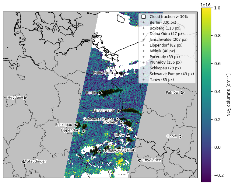
The code computes several new fields that are added to the provided data dataset. The detected plumes are stored in the detected_plume data array (dims: nobs, nrows, source) where the length of source is equal to the number of detected plumes.
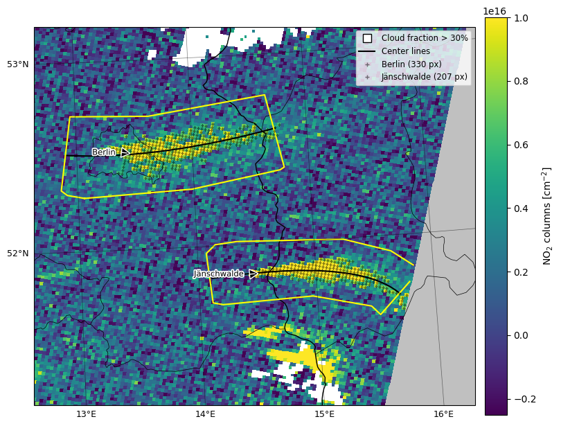
The plume detection can be visualized using the ddeq.vis.show_level2 function:
[10]:
fig = ddeq.vis.show_level2(data, data['NO2'], gas='NO2', domain=DOMAIN, sources=sources,
                           winds=winds, do_zoom=False, show_clouds=True)
Exercise
Detect emission plumes Berlin and Jänschwalde using low-noise CO2 observations.
Increase the size of the Gaussian filter to increase number of detected pixels.
Visualize the results using
ddeq.vis.show_level2
[ ]:
Center lines and polygons
To estimate emissions for detected plumes, the following code fits a center curve for each detected plume. The code also adds across- and along-plume coordinates (xp and yp). The computation of plume coordinates can result in multiple solutions when the center line is strongly curved or the plume is small.
[11]:
# Read SMARTCARB Level-2 file
filename = os.path.join(DATA_PATH, 'Sentinel_7_CO2_2015042311_o1670_l0483.nc')
data = ddeq.smartcarb.read_level2(
    filename, co2_noise_scenario='low', no2_noise_scenario='high',
    co_noise_scenario='low', only_observations=False
)

# Detect plumes using NO2 observations
data = ddeq.dplume.detect_plumes(
    data, sources.sel(source=['Berlin', 'Janschwalde']), crs=CRS,
    variable='NO2', variable_std='NO2_std',
    filter_type='gaussian', filter_size=0.5
)

# Fit center curve to detected plumes
data = ddeq.curves.fit_to_detections(data, n_nodes=3, force_origin=True, use_weights=True)

# Compute natural coordinates of along and across plume direction for each plume:
data = ddeq.curves.compute_natural_coords(data)

# Define areas around plume
data = ddeq.curves.compute_plume_areas(data)
The following code shows the result:
[12]:
ddeq.vis.show_level2(
    data, 'NO2', gas="NO2", domain=DOMAIN, winds=winds, do_zoom=True,
    show_clouds=True, draw_gridlines=True, crs=CRS
);
Prepare emission quantification
To prepare for estimating the emissions the following code computes the CO2 and NO2 background field, the plume signals and converts to mass columns in kg/m² using the ucat Python package.
[13]:
for gas in ["CO2", "NO2"]:

    # estimate background
    data = ddeq.background.estimate(data, gas)

    # compute CO2/NO2 enhancement
    data = ddeq.emissions.compute_plume_signal(data, gas)

    # convert ppm to kg/m2
    for variable in [
        gas,
        f"{gas}_estimated_background",
        f"{gas}_minus_estimated_background",
    ]:
        ddeq.emissions.convert_units(data, gas, variable)
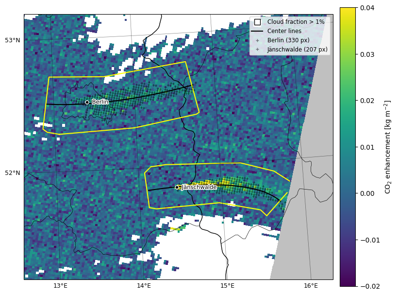
It is possible to visualize different variables using the variable parameter:
[14]:
ddeq.vis.show_level2(
    data, 'CO2_minus_estimated_background_mass', gas='CO2', domain=DOMAIN,
    winds=None, do_zoom=True, show_clouds=True, draw_gridlines=True,
    vmin=-20e-3, vmax=40e-3,
    label='CO$_2$ enhancement [kg m$^{-2}$]', crs=CRS
);
Cross-sectional flux method
The following code estimated CO\(_2\) and NO\(_x\) emissions for a point source (Jänschwalde) and a city (Berlin):
True emissions
The SMARTCARB dataset has the true emissions, which can be read for a CO2M dataset by provding the time:
[15]:
sources = ddeq.sources.read_smartcarb(time=data.time)
sources
[15]:
<xarray.Dataset> Size: 1kB
Dimensions:                  (source: 16)
Coordinates:
  * source                   (source) object 128B 'Berlin' 'Boxberg' ... 'Turow'
Data variables:
    label                    (source) object 128B 'Berlin' 'Boxberg' ... 'Turów'
    lon                      (source) float64 128B 13.41 14.57 ... 8.957 14.91
    lat                      (source) float64 128B 52.52 51.42 ... 50.09 50.94
    diameter                 (source) int64 128B 30000 1000 1000 ... 1000 1000
    CO2_emissions            (source) float64 128B 534.6 604.1 ... 156.2 276.3
    NOx_emissions            (source) float64 128B 0.5767 0.4878 ... 0.4156
    CO2_emissions_precision  (source) float64 128B 226.4 139.7 ... 43.6 63.92
    NOx_emissions_precision  (source) float64 128B 0.204 0.1126 ... 0.09596
    true_CO2_emissions       (source) float64 128B 742.4 768.3 ... 194.7 351.5
    true_NOx_emissions       (source) float64 128B 0.7972 0.62 ... 0.1501 0.5282
Attributes:
description: Cities and power plants inside the SMARTCARB model domain.Cross-sectional flux method for point source
Wind speed and direction are taken from ERA-5 data that are downloaded from the Copernicus Climate Data Store (CDS). This can be done automatically using cdsapi but requires a CDS account and it might be slow especially when downloading ERA-5 on model levels.
In the example below, winds are computed from ERA-5 on model levels using the GNFR-A emission profile for vertical averaging. A subset of ERA-5 data from the SMARTCARB model domain is included in DATA_PATH for testing.
[16]:
lvl_filename = os.path.join(DATA_PATH, "SMARTCARB_ERA5-lvl-20150423t1100.nc")
sng_filename = os.path.join(DATA_PATH, "SMARTCARB_ERA5-sfc-20150423t1100.nc")

winds = ddeq.era5.read(sng_filename, lvl_filename, method="GNFR_A", sources=sources, times=data.time)
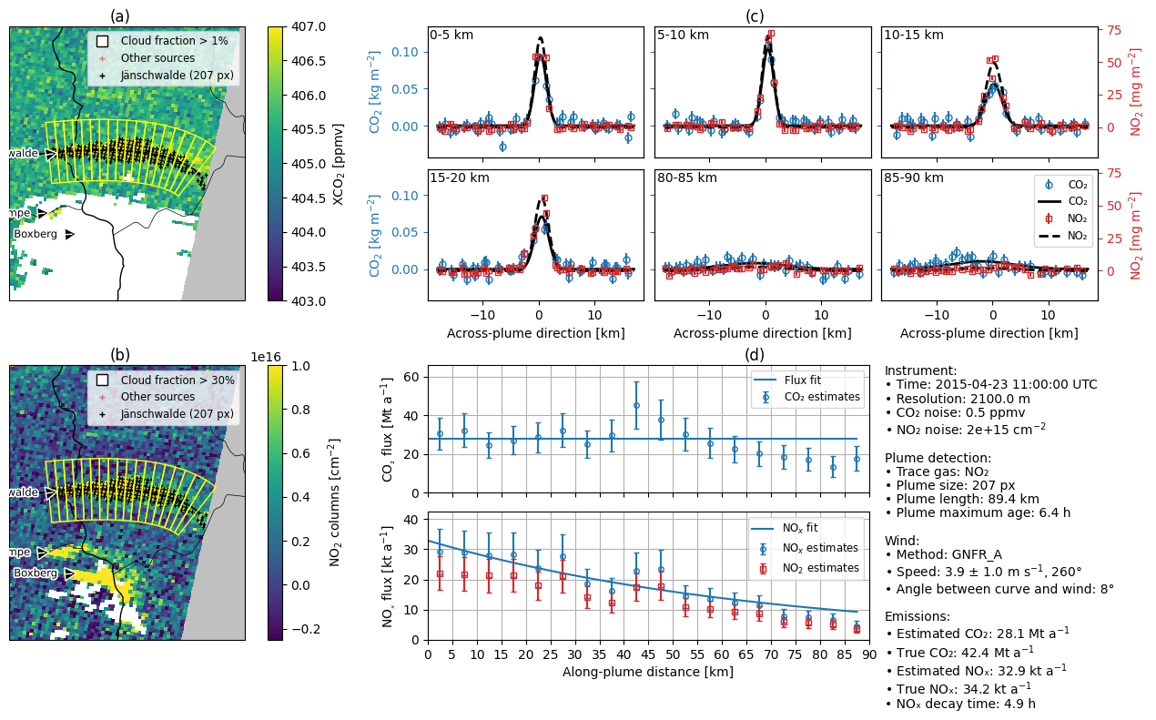
The cross-sectional flux (csf) method is performed by the following function.
Note that f_model gives the factor for converting NO2 to NOx line densities.
[17]:
results = ddeq.csf.estimate_emissions(
    data,
    winds,
    sources.sel(source=["Janschwalde"]),
    xmin=0,           # position downstream of the first polygon for computing fluxes
    xmax=np.inf,      # position of the last polygon (maximum plume length)
    dx=5e3,           # width of polygons in along-plume direction
    method='gauss',
    gases=['CO2', 'NO2'],
    crs=CRS,
    f_model=1.32
)
/home/docs/checkouts/readthedocs.org/user_builds/ddeq/envs/v1.1/lib/python3.12/site-packages/ddeq/csf.py:1098: FutureWarning: In a future version of xarray the default value for data_vars will change from data_vars='all' to data_vars=None. This is likely to lead to different results when multiple datasets have matching variables with overlapping values. To opt in to new defaults and get rid of these warnings now use `set_options(use_new_combine_kwarg_defaults=True) or set data_vars explicitly.
  polygons = xr.concat(
The results can be visualized with the following function:
[18]:
with xr.set_options(keep_attrs=True):
    fig = ddeq.vis.plot_csf_result(
        ['CO2', 'NO2'],
        data, winds, results,
        source='Janschwalde',
        sources=sources,
        domain=DOMAIN, crs=CRS
    )
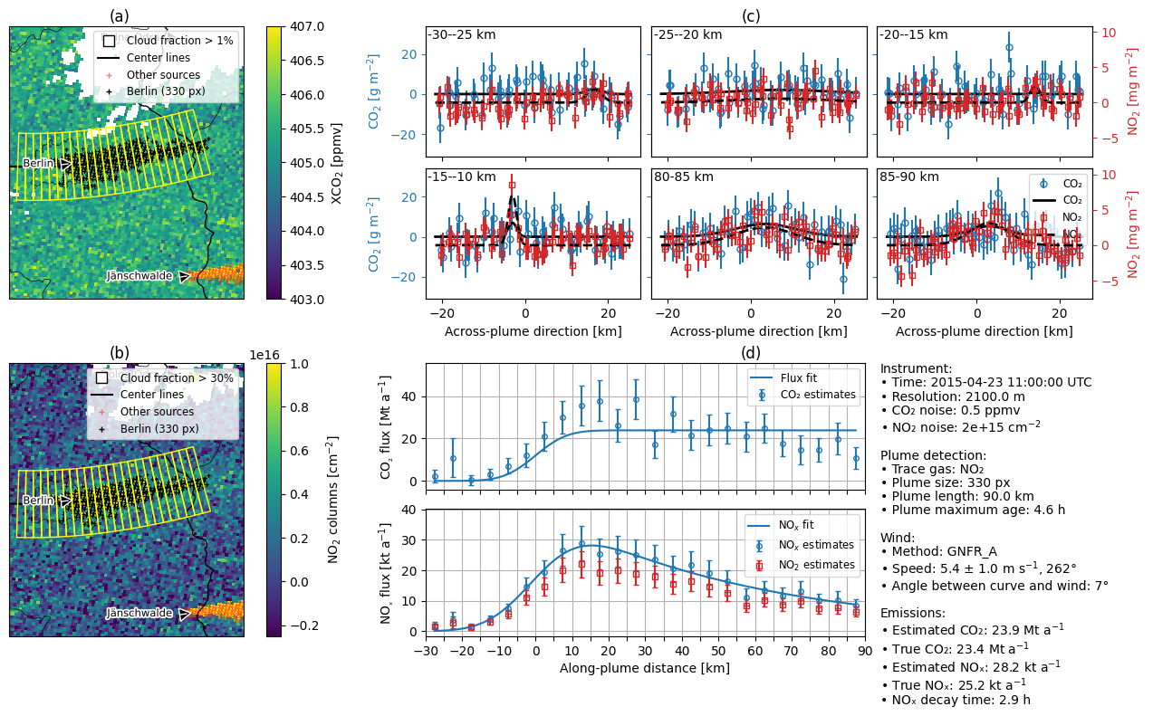
Cross-sectional flux method for a city
The cross sectional flux method over a city is slightly different, because the flux slowly builds up over the city area. For NO\(_x\), fluxes over the city are therefore modeled by a Gaussian curve.
[19]:
results = ddeq.csf.estimate_emissions(
    data,
    winds,
    sources.sel(source=["Berlin"]),
    xmin=-30e3,       # position downstream of the first polygon for computing fluxes
    xmax=np.inf,      # position of the last polygon (maximum plume length)
    dx=5e3,           # width of polygons in along-plume direction
    method='gauss',
    gases=['CO2', 'NO2'],
    crs=CRS,
    f_model=1.32,
)

fig = ddeq.vis.plot_csf_result(
    ['CO2', 'NO2'],
    data,
    winds,
    results,
    sources=sources,
    source='Berlin',
    domain=DOMAIN, crs=CRS,
)
/home/docs/checkouts/readthedocs.org/user_builds/ddeq/envs/v1.1/lib/python3.12/site-packages/ddeq/csf.py:1098: FutureWarning: In a future version of xarray the default value for data_vars will change from data_vars='all' to data_vars=None. This is likely to lead to different results when multiple datasets have matching variables with overlapping values. To opt in to new defaults and get rid of these warnings now use `set_options(use_new_combine_kwarg_defaults=True) or set data_vars explicitly.
  polygons = xr.concat(
Exercise
Write code to quantify the CO2 and NOx emissions of other point sources.
[ ]:
Integrated mass enhancement
The following code uses integrated mass enhancement for computing CO\(_2\) emissions. First, the wind field is extracted from the SMARTCARB dataset at each source location. Second, the IME method is applied to estimate the emissions.
[20]:
winds = ddeq.wind.read_smartcarb(time, sources.lon, sources.lat, data_path=DATA_PATH)
[21]:
results = ddeq.ime.estimate_emissions(data, winds, sources, gas='CO2')

print(' ' * 10, '\tEstimate\tTrue')

for name, source in sources.groupby('source'):
    if name in data.source:
        Q = results['CO2_emissions'].sel(source=name).values
        Q_true = ddeq.smartcarb.read_true_emissions(
            time=pd.Timestamp(data.time.values), gas='CO2', source=name
        ).mean()
        print(
            f'{name:10s}\t'
            f'{ucat.convert_mass_per_time_unit(Q, "kg/s", "Mt/a"):.1f} Mt/a\t'
            f'{ucat.convert_mass_per_time_unit(Q_true, "kg/s", "Mt/a"):.1f} Mt/a'
        )
                Estimate        True
Berlin          19.3 Mt/a       23.4 Mt/a
Janschwalde     43.4 Mt/a       42.4 Mt/a
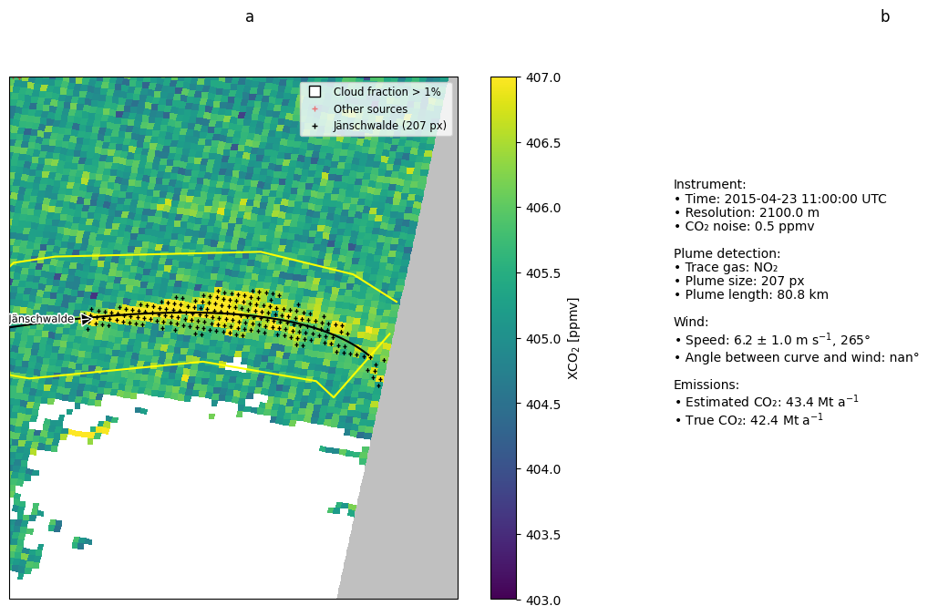
The results can be visualized with the following function:
[22]:
Q_true = ddeq.smartcarb.read_true_emissions(
    time=pd.Timestamp(data.time.values),
    gas='CO2',
    source='Janschwalde'
).mean()

with xr.set_options(keep_attrs=True):
    fig = ddeq.vis.plot_ime_result(
        'CO2',
        data, winds, results,
        source='Janschwalde',
        domain=DOMAIN, crs=CRS,
        true_emissions=Q_true,
        do_zoom=True,
    )
[23]:
results = ddeq.ime.estimate_emissions(data, winds, sources,
                                      gas='NO2', decay_time=4*60**2)

results = ddeq.emissions.convert_NO2_to_NOx_emissions(results, f=1.32)

print(' ' * 10, '\tEstimate\tTrue')

for name, source in sources.groupby('source'):
    if name in data.source:
        Q = results['NOx_emissions'].sel(source=name).values
        Q_true = ddeq.smartcarb.read_true_emissions(
            time=pd.Timestamp(data.time.values), gas='NO2', source=name
        ).mean()
        print(
            f'{name:10s}\t'
            f'{ucat.convert_mass_per_time_unit(Q, "kg/s", "kt/a"):.1f} Mt/a\t'
            f'{ucat.convert_mass_per_time_unit(Q_true, "kg/s", "kt/a"):.1f} Mt/a'
        )
                Estimate        True
Berlin          31.2 Mt/a       25.2 Mt/a
Janschwalde     46.1 Mt/a       34.2 Mt/a
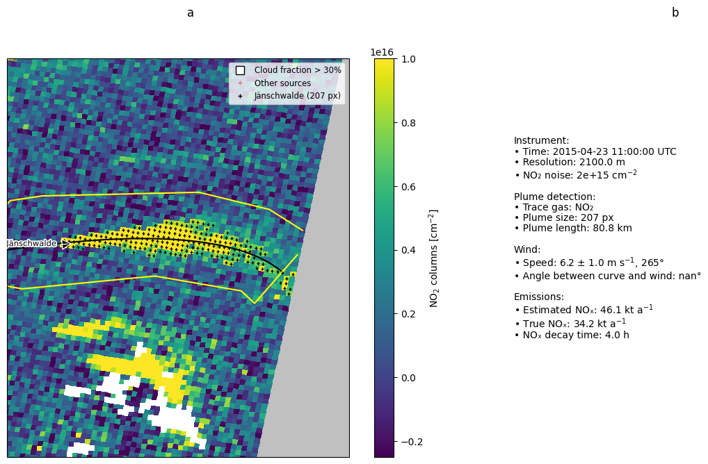
[24]:
Q_true = ddeq.smartcarb.read_true_emissions(
    time=pd.Timestamp(data.time.values),
    gas='NOx',
    source='Janschwalde'
).mean()

with xr.set_options(keep_attrs=True):
    fig = ddeq.vis.plot_ime_result(
        'NO2',
        data, winds, results,
        source='Janschwalde',
        domain=DOMAIN, crs=CRS,
        true_emissions=Q_true,
        do_zoom=True,
    )
[ ]: