Example: TROPOMI NO\(_2\) plume
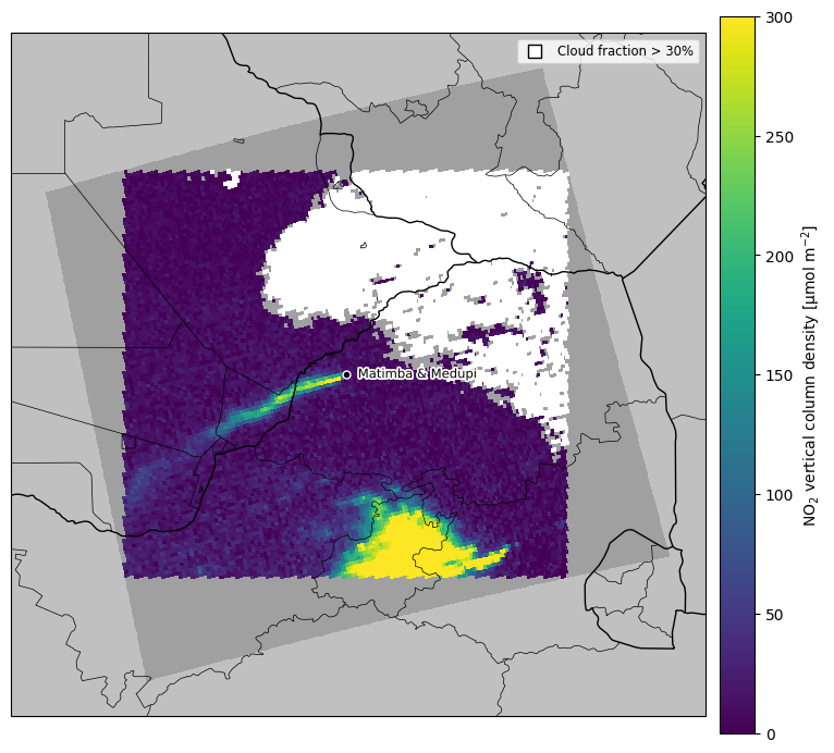
An example demonstrating the application of the CSF and Gaussian plume inversion for estimating NOx emissions from the Matimba/Medupi power plant using TROPOMI NO2 images.
[1]:
import os

import cartopy.crs as ccrs
import matplotlib.pyplot as plt
import numpy as np
import pandas as pd
import ucat
import xarray as xr

import ddeq

sources = ddeq.misc.read_point_sources()
sources = sources.sel(source=['Matimba'])

filename = os.path.join(ddeq.DATA_PATH, 'Matimba_S5P_RPRO_L2__NO2____20210725T110715.nc')

DOMAIN = ddeq.misc.Domain('Matimba', 25, -25.2, 29, -22.9)
CRS = ddeq.misc.get_opt_crs(DOMAIN)

CURVE_STYLE = "BEZIER"     # "POLY" or "BEZIER"
DETECTION = "THR"         # "THR" or "WIND"
BACKGROUND = "LINEAR"      # "LINEAR" or "SMOOTH"
2025-12-04 09:16:01.001243703 [W:onnxruntime:Default, device_discovery.cc:164 DiscoverDevicesForPlatform] GPU device discovery failed: device_discovery.cc:89 ReadFileContents Failed to open file: "/sys/class/drm/card0/device/vendor"
Sentinel-5P/TROPMI NO2 dataset
[2]:
data = xr.open_dataset(filename)
[3]:
fig = ddeq.vis.show_level2(
    data, 1e6 * data['NO2'],
    sources=sources,
    vmin=0,
    vmax=300,
    label="NO$_2$ vertical column density [µmol m$^{-2}$]", do_zoom=True,
    units='umol m-2'
)
ERA5 wind files
The code below would download ERA5 single level and pressure level. Since the files are already in ddeq.DATA_PATH, no files will be downloaded. If you want to download own ERA5 data, please the change data_path to the location on your system, where you like to save your files.
[4]:
sng_filename = ddeq.era5dl.download_single_lvl(
    time=pd.Timestamp(data.time.values),
    area=DOMAIN.extent,
    timesteps=24,
    data_path=ddeq.DATA_PATH,
    prefix="Matimba"
)

lvl_filename = ddeq.era5dl.download_pressure_lvl(
    time=pd.Timestamp(data.time.values),
    area=DOMAIN.extent,
    timesteps=24,
    data_path=ddeq.DATA_PATH,
    prefix="Matimba"
)

sng_filename, lvl_filename
[4]:
('/home/docs/checkouts/readthedocs.org/user_builds/ddeq/envs/stable/lib/python3.12/site-packages/ddeq/data/Matimba_ERA5-sl-20210725.nc',
 '/home/docs/checkouts/readthedocs.org/user_builds/ddeq/envs/stable/lib/python3.12/site-packages/ddeq/data/Matimba_ERA5-pl-20210725.nc')
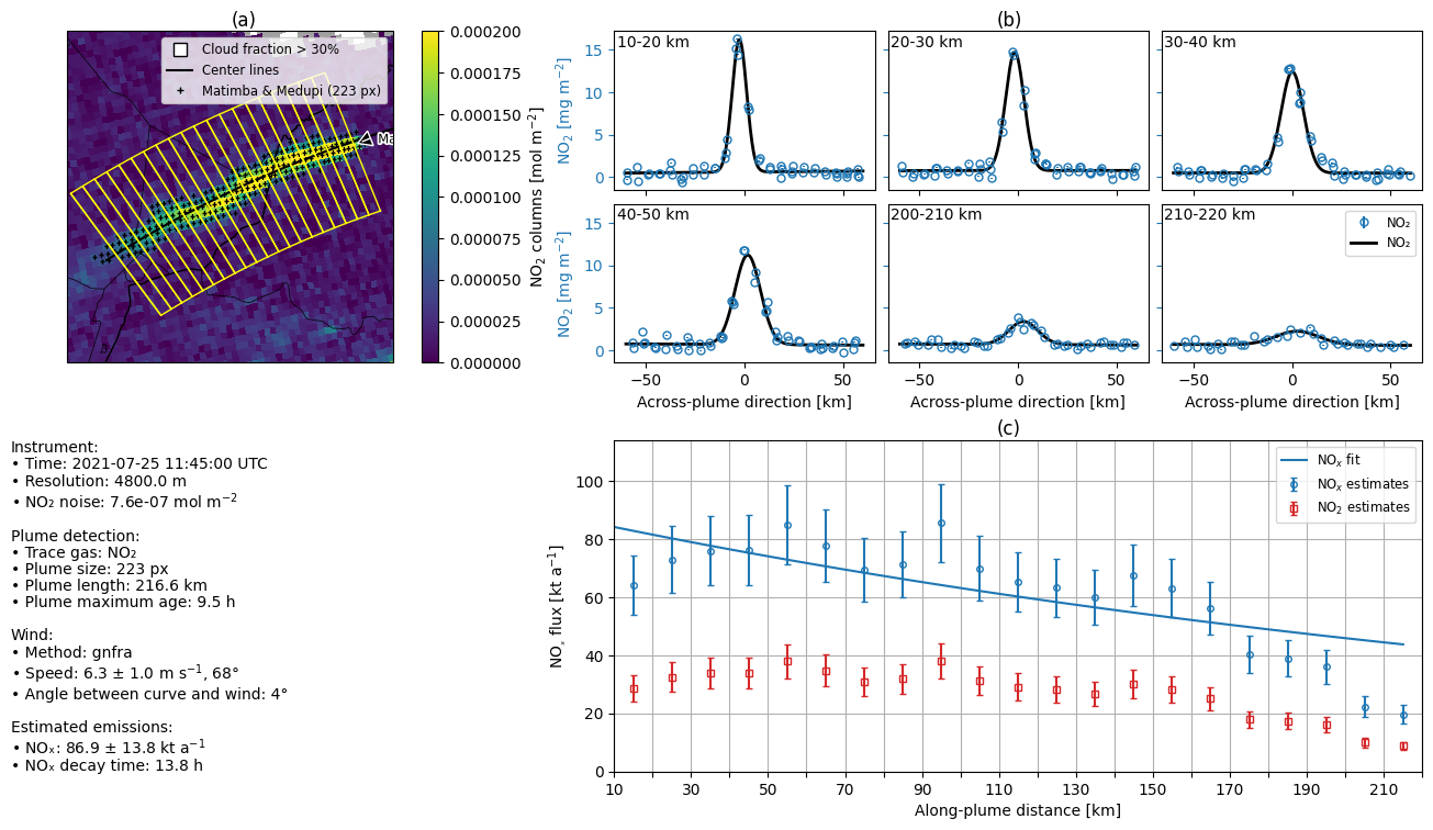
Cross-sectional flux method
[5]:
# Effective wind at source locations using GNFR-A weighted winds:
winds = ddeq.era5.read(
    sng_filename,
    lvl_filename,
    method="gnfra",
    sources=sources,
    times=data.time
)
winds
[5]:
<xarray.Dataset> Size: 96B
Dimensions:          (time: 1, source: 1)
Coordinates:
  * time             (time) datetime64[ns] 8B 2021-07-25T11:44:52.595066640
  * source           (source) object 8B 'Matimba'
    number           int64 8B 0
    expver           (time) <U4 16B '0001'
    lon              (source) float64 8B 27.61
    lat              (source) float64 8B -23.67
Data variables:
    U                (time, source) float64 8B -5.856
    V                (time, source) float64 8B -2.344
    speed            (time, source) float64 8B 6.308
    speed_precision  (time, source) float64 8B 1.0
    direction        (time, source) float64 8B 68.18
Attributes:
    CREATOR:       ddeq.era5
    DATE_CREATED:  2025-12-04 09:16
    ORIGIN:        ERA-5
    METHOD:        gnfra
DESCRIPTION: Weighted average for U- and V-wind using GNFR-A emission p...[6]:
if DETECTION == "THR":

    var_sys = (ucat.convert_columns(0.5e15, 'cm-2', 'mol m-2',
                                    molar_mass='NO2'))**2

    data = ddeq.dplume.detect_plumes(data, sources,
                                     variable='NO2',
                                     variable_std='NO2_std',
                                     var_sys=var_sys,
                                     filter_type='gaussian',
                                     filter_size=0.5, crs=CRS)
elif DETECTION == "WIND":
    data = ddeq.dplume.detect_from_wind(data, sources, winds, dmax=30e3, crs=CRS)
else:
    raise ValueError
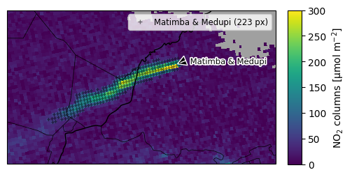
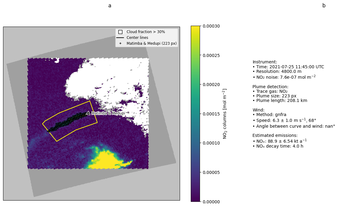
[7]:
fig = ddeq.vis.show_level2(
    data, 1e6 * data['NO2'], gas='NO2',
    vmin=0,
    vmax=300,
    label="NO$_2$ columns [µmol m$^{-2}$]",
    winds=winds,
    domain=DOMAIN,
    do_zoom=False, show_clouds=False, crs=CRS,
    figwidth=4,
);
[8]:
variable = "NO2_mass"
background = "linear"
ddeq.emissions.convert_units(data, "NO2", "NO2")
[9]:
if DETECTION == "THR":
    data = ddeq.curves.fit_to_detections(data, n_nodes=3, force_origin=True, use_weights=True)

data = ddeq.curves.compute_natural_coords(data)
data = ddeq.curves.compute_plume_areas(data, plume_width=120e3)

# estimate NO2 enhancement
ddeq.background.estimate(data, "NO2")
ddeq.emissions.compute_plume_signal(data, "NO2")

ddeq.emissions.convert_units(data, "NO2", "NO2_estimated_background")
ddeq.emissions.convert_units(data, "NO2", "NO2_minus_estimated_background")
[10]:
dx = None if DETECTION == "WIND" else 10e3

results_csf = ddeq.csf.estimate_emissions(data, winds, sources, 'NO2',
                                          xmin=10e3, dx=dx,
                                          f_model=2.24, crs=CRS,
                                          variable=variable, background=background
                                         )
/home/docs/checkouts/readthedocs.org/user_builds/ddeq/envs/stable/lib/python3.12/site-packages/ddeq/csf.py:1098: FutureWarning: In a future version of xarray the default value for data_vars will change from data_vars='all' to data_vars=None. This is likely to lead to different results when multiple datasets have matching variables with overlapping values. To opt in to new defaults and get rid of these warnings now use `set_options(use_new_combine_kwarg_defaults=True) or set data_vars explicitly.
  polygons = xr.concat(
[11]:
ddeq.vis.plot_csf_result(['NO2'], data, winds, results_csf, 'Matimba',
                         vmins=[0], vmaxs=[200e-6], crs=CRS);
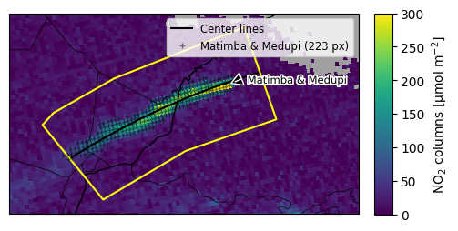
[12]:
fig = ddeq.vis.show_level2(
    data,
    1e6 * data['NO2'],
    gas='NO2',
    vmin=0,
    vmax=300,
    label="NO$_2$ columns [µmol m$^{-2}$]",
    winds=winds,
    domain=DOMAIN,
    do_zoom=False,
    show_clouds=False,
    crs=CRS,
    figwidth=4,
);
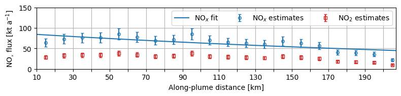
[13]:
fig, ax  = plt.subplots(1, figsize=(8,2))
ddeq.vis.plot_along_plume(ax, 'NO2', results_csf.sel(source='Matimba'))
ax.set_xlim(right=207)
ax.set_ylim(0,150)
plt.tight_layout()

ax.legend().remove()
ax.legend(loc=1, ncol=3)
[13]:
<matplotlib.legend.Legend at 0x7d8b99ba1520>
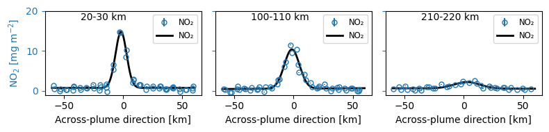
[14]:
fig, axes  = plt.subplots(1,3, figsize=(8,2), sharey=True)


for i, ax in zip([1,9,-1], axes):
    try:
        r = results_csf.sel(source='Matimba').isel(polygon=i)
    except IndexError:
        continue
    ddeq.vis.plot_across_section(r, gases=['NO2'], method='gauss', ax=ax,
                                 legend='simple')

    ax.text(-36, 19.5, '%d-%d km' % (r.xa/1e3, r.xb/1e3), ha='left', va='top')

for ax in axes[1:]:
    ax.set_ylim(-1, 20)
    ax.set_ylabel('')


plt.tight_layout()
[15]:
ddeq.vis.plot_csf_result(['NO2'], data, winds, results_csf, 'Matimba',
                         vmins=[0], vmaxs=[200e-6], crs=CRS);

Gaussian plume inversion
[16]:
priors = {'Matimba': {
    'NO2': {'Q': 3.0,       # kg/s
            'tau': 4*60**2  # seconds
           }
}}
data, results_gauss = ddeq.gauss.estimate_emissions(data, winds, sources,
                                                    ['NO2'], priors=priors,
                                                    fit_decay_times=True)
[17]:
results_gauss = ddeq.emissions.convert_NO2_to_NOx_emissions(results_gauss, f=2.38)
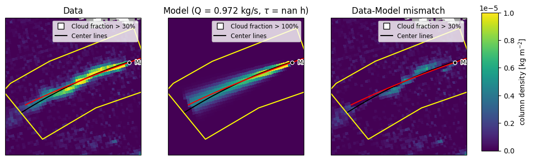
[18]:
fig = ddeq.vis.plot_gauss_result(data, results_gauss, ['Matimba'],
                                 'NO2', crs=CRS, vmin=0, vmax=10e-6)
IME method
[19]:
results_ime = ddeq.ime.estimate_emissions(
    data,
    winds,
    sources,
    "NO2",
    decay_time=4.0*60**2
)
results_ime = ddeq.emissions.convert_NO2_to_NOx_emissions(results_ime, f=1.32)
[20]:
ddeq.vis.plot_ime_result(
    "NO2",
    data,
    winds,
    results_ime,
    "Matimba",
    crs=CRS,
    vmin=0,
    vmax=300e-6,
);
LCSF method
Quick example applying the LCSF method to TROPOMI NO2 data
[21]:
# Convert from mol/m2 to molec/cm2 for LCSF method
data["NO2"] = ucat.convert_columns(data["NO2"], "mol/m2", "cm-2")
data["NO2_std"] = ucat.convert_columns(data["NO2_std"], "mol/m2", "cm-2")
[22]:
wind_field = ddeq.era5.read(
    sng_filename,
    lvl_filename,
    method="gnfra",
    times=data.time
)
[23]:
lcs_params = {}
lcs_params['use_prior'] = True
lcs_params["verbose"] = True

lcs_params['n_min_fit_pts'] = 10
lcs_params['fit_pt_slice_width'] = 15

lcs_params['f_NOx_NO2'] = 3.5
lcs_params['NOx_NO2_tau_depletion'] = 4.0 * 60**2

lcsf_results = ddeq.lcsf.estimate_emissions(data, wind_field, sources, ['NO2'], priors=priors, lcs_params=lcs_params, all_diags=True)
print(f"NOx emissions: {np.nanmedian(lcsf_results['NO2_emissions']):.1f} kt NO2 / a")
LCSF parameters
{'use_prior': True, 'verbose': True, 'n_min_fit_pts': 10, 'fit_pt_slice_width': 15, 'f_NOx_NO2': 3.5, 'NOx_NO2_tau_depletion': 14400.0, 'min_estim_emis': None, 'max_estim_emis': None, 'Enhancement_thresh': 1.0, 'max_sigma_Gauss': 5.0, 'max_rel_std_emis': 1.0, 'window_length': 100}

**************

Estimating line densities and emissions for source Matimba

10 LD found !
NO2 median emission estimate  101.68162
NOx emissions: 101.7 kt NO2 / a
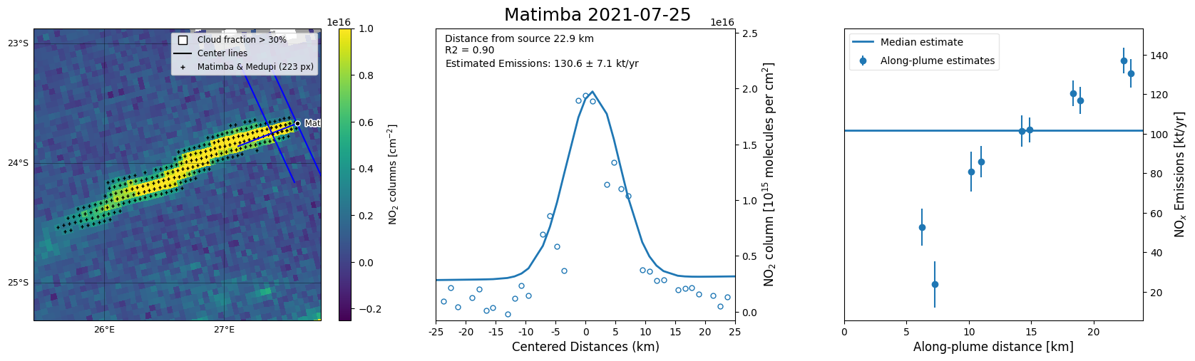
[24]:
fig = ddeq.vis.plot_lcsf_result("Matimba", lcsf_results, data, sources,
                                gases=['NO2'])
/home/docs/checkouts/readthedocs.org/user_builds/ddeq/envs/stable/lib/python3.12/site-packages/ddeq/vis.py:1097: UserWarning: To plot the polygons, a coordinate reference system (crs) must be provided.
  warnings.warn(
[ ]: